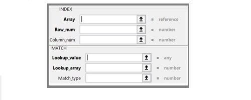
To find the Index Match is one of the important and widely used functions in excel. It is used for performing advanced lookup functions. Index and Match function can be used separately, but they are generally used in tandem.
How is Index Match function different from Vlookup?
Vlookup allows us to perform the only one-way lookup, and the lookup value should always be in the first column of the table array. See how Vlookup is used.
On the contrary, the Index and Match function is extremely flexible. It allows us to perform horizontal and vertical lookups, 2-way lookups, left lookups, and even lookups based on multiple criteria.
Index Function
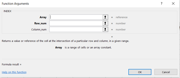
Index basically retrieves the value at a given location in the range. And the range can be one-dimensional or two dimensional. Let’s first understand the components of the Index function.
Array: It is a range from where we have to retrieve the value.
Row Number: From which row we want to retrieve the value.
Column Number: From which column we want to retrieve the value.
One-Dimensional Range (Company Name)
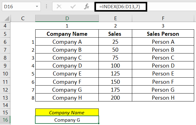
Given below is the dataset that comprises of Company Name, Sales, and Corresponding Sales Person.
Suppose from the given dataset we want the name of the 7th company. So, we can use the Index formula as highlighted in the image below. Here, the range is D6:D13, and 7 is the row number of the table array.
Two-Dimensional Range (Company Name and Sales)
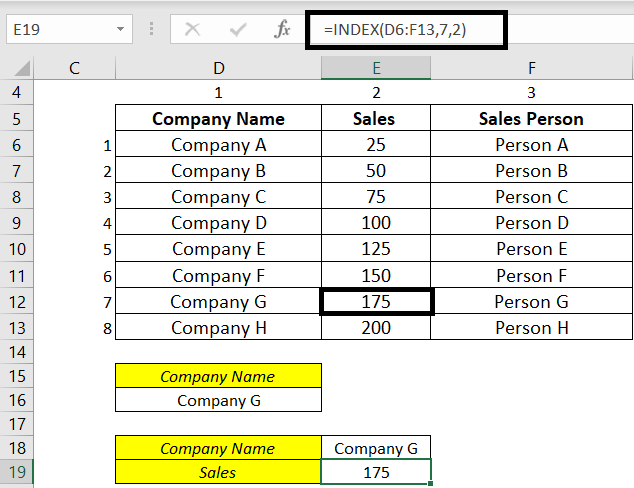
Now, suppose we want sales of Company G. We can use the Index formula as highlighted in the below image. It takes row and column as input with the data table and gives an output of intersection. In this example, the intersection of row 7 and column 2 is cell E12.
***** FinShiksha Learning Championship 2021 – Details here ******
Match Function
We need to use the Match function to find the position of value in the range. It can find a position in a horizontal or vertical array. Let’s understand the components of the Match function.
Lookup Value: It is basically the value for which we want the position in the range.
Lookup Array: It is a range where value is used.
Match Type: 0 for Exact match, +1 or -1 for approximate match
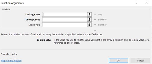
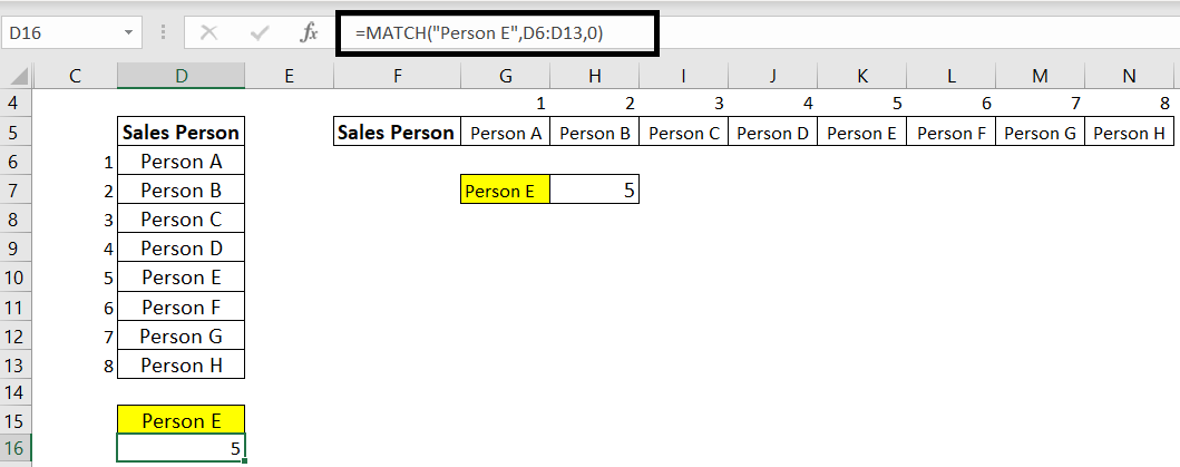
Below dataset gives salesperson, and we want to find the position of Person E.
For the vertical array, we can use the match function as highlighted in the below image. Range D6:D13 is in this example.
For horizontal array, we can use the Match function as follows. Range G5:N5 is used in this example.
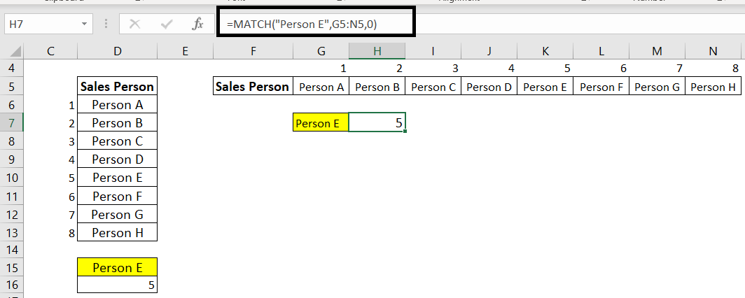
Note: In the above example, we have used an exact match. For the lookup value, we have used Person E in the formula. Alternatively, we can give a cell reference instead of Person E.
Index and Match Combined
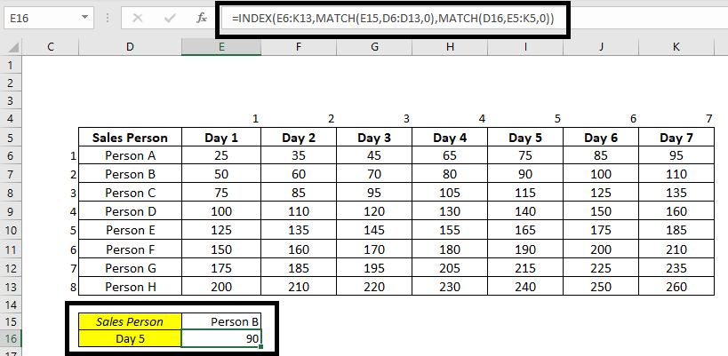
Let’s understand this with the help of an example. Dataset of 7 days of sales made by different salesperson and we have to find out the sales made by Person B on Day 5.
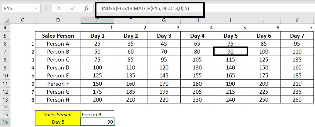
We can use the Index function for that and give the range as E6:K13 with row number 2 and column number 5 of the table array.
=INDEX(E6:K13,2,5)
It will return the value of 90.
To make this formula dynamic, we can use the Match function with the Index function as highlighted in the above snapshot. The match function will search for Person B in the row, and the Index function will retrieve the value of the point of intersection of Person B and Day 5 as we have given column 5 as an input.
Curious to explore this!!! Index_Match_Part1
To stay updated about all of our posts and webinars on Businesses and Finance Careers – register and create a free account on our website. You will also get access to a free Finance Bootcamp course once you register.
Other Blogs in the Excel Series – Vlookup Function | Dynamic Dropdown Function


