Wondering where and how to use Dynamic Dropdown function? We have often encountered a situation where we need to select a particular value from the dropdown menu. Dropdown is easy to create in excel. However, in this post, we will explore the possibility to create a dynamic dropdown – which means the value of the dropdown menu will change based on the selection.

Before we deep down further, let’s see how to create a simple dropdown menu.

Dataset comprises of Department and Executives from those departments. You can download Dynamic Dropdown excel.

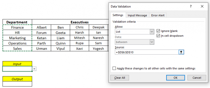
If we look at the excel, then the Departments are mentioned in the D6 to D10 range. And we want to create a dropdown containing the list in cell D14.

Method to use dynamic dropdown function:

Go to Data Tab > Go to Data Tools Section > Click on Data Validation > Select List.

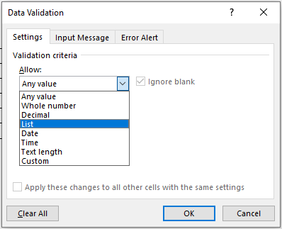
Once the “List Option” is selected, Excel will ask you to provide the data range. When you click OK, the dropdown list will be created (as you can see in the below picture – Input cell)

Problem Statement for dynamic dropdown function?

We want another dropdown list in the output field, and that list should contain the name of the executives from a particular department (which is selected as an input).

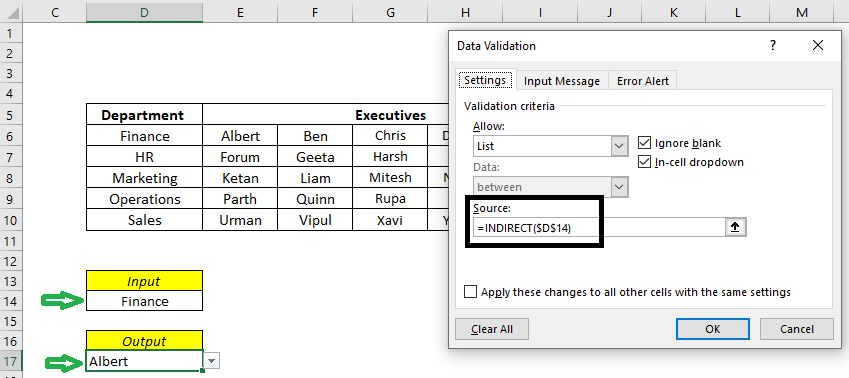
That is where we can use a function called INDIRECT.

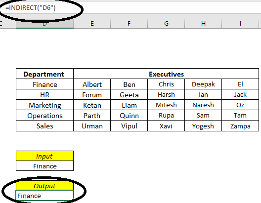
What is the INDIRECT function? This function returns a valid reference from a given text string. In a simple language, we can provide a cell reference, and it will return a cell value. (see picture below)

Over here, the formula has taken D6 as a reference, and the output is the value contained by cell D6 (which is “Finance”)

But the INDIRECT function will only give one output – so how do we turn it to provide multiple outputs.

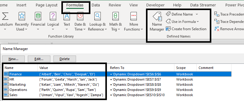
This is where we use NAME MANAGER. We will convert the respective Department name as a Name and then use the INDIRECT function to reference this Name.

*****    FinShiksha Learning Championship 2021 – Details here   ******

How to create a Name?

Select the range and provide a name directly.

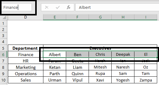
Do this activity for all departments. And you can see all created names in Name Manager (Go To Formulas Tab > Defined Names Section > Name Manager.

Once the above activity is done, then go to cell D17 and create a list.

Curious to explore this!!! Dynamic Dropdown Excel

To stay updated about all of our posts and webinars on Businesses and Finance Careers – register and create a free account on our website. You will also get access to a free Finance Bootcamp course once you register.

Other Blogs in the Excel Series – Vlookup Function